Differential equation how to solve

Differential Equations

You appear to be on a device with a "narrow" screen width (i.e. you are probably on a mobile phone). Due to the nature of the mathematics on this site it is best views in landscape mode. If your device is not in landscape mode many of the equations will run off the side of your device (should be able to scroll to see them) and some of the menu items will be cut off due to the narrow screen width.

Section 2-1 : Linear Differential Equations

The first special case of first order differential equations that we will look at is the linear first order differential equation. In this case, unlike most of the first order cases that we will look at, we can actually derive a formula for the general solution. The general solution is derived below. However, we would suggest that you do not memorize the formula itself. Instead of memorizing the formula you should memorize and understand the process that I'm going to use to derive the formula. Most problems are actually easier to work by using the process instead of using the formula.
So, let's see how to solve a linear first order differential equation. Remember as we go through this process that the goal is to arrive at a solution that is in the form y=y(t). It's sometimes easy to lose sight of the goal as we go through this process for the first time.
In order to solve a linear first order differential equation we MUST start with the differential equation in the form shown below. If the differential equation is not in this form then the process we’re going to use will not work.
dydt+p(t)y=g(t)$$\begin{array}{}\frac{dy}{dt}+p\left(t\right)y=g\left(t\right)& \text{(1)}\end{array}$$Where both p(t) and g(t) are continuous functions. Recall that a quick and dirty definition of a continuous function is that a function will be continuous provided you can draw the graph from left to right without ever picking up your pencil/pen. In other words, a function is continuous if there are no holes or breaks in it.
Now, we are going to assume that there is some magical function somewhere out there in the world, μ(t), called an integrating factor. Do not, at this point, worry about what this function is or where it came from. We will figure out what μ(t) is once we have the formula for the general solution in hand.
So, now that we have assumed the existence of μ(t) multiply everything in (1) by μ(t). This will give.
μ(t)dydt+μ(t)p(t)y=μ(t)g(t)$$\begin{array}{}\mu \left(t\right)\frac{dy}{dt}+\mu \left(t\right)p\left(t\right)y=\mu \left(t\right)g\left(t\right)& \text{(2)}\end{array}$$Now, this is where the magic of μ(t) comes into play. We are going to assume that whatever μ(t) is, it will satisfy the following.
μ(t)p(t)=μ′(t)$$\mu \left(t\right)p\left(t\right)={\mu }^{\prime }\left(t\right)$$Again do not worry about how we can find a μ(t) that will satisfy (3). As we will see, provided p(t) is continuous we can find it. So substituting (3) we now arrive at.
μ(t)dydt+μ′(t)y=μ(t)g(t)$$\mu \left(t\right)\frac{dy}{dt}+{\mu }^{\prime }\left(t\right)y=\mu \left(t\right)g\left(t\right)$$At this point we need to recognize that the left side of (4) is nothing more than the following product rule.
μ(t)dydt+μ′(t)y=(μ(t)y(t))′$$\mu \left(t\right)\frac{dy}{dt}+{\mu }^{\prime }\left(t\right)y={\left(\mu \left(t\right)y\left(t\right)\right)}^{\prime }$$So we can replace the left side of (4) with this product rule. Upon doing this (4) becomes
(μ(t)y(t))′=μ(t)g(t)$${\left(\mu \left(t\right)y\left(t\right)\right)}^{\prime }=\mu \left(t\right)g\left(t\right)$$Now, recall that we are after y(t). We can now do something about that. All we need to do is integrate both sides then use a little algebra and we'll have the solution. So, integrate both sides of (5) to get.
∫(μ(t)y(t))′dt=∫μ(t)g(t)dt$$\int {\left(\mu \left(t\right)y\left(t\right)\right)}^{\prime }dt=\int \mu \left(t\right)g\left(t\right)dt$$μ(t)y(t)+c=∫μ(t)g(t)dt$$\mu \left(t\right)y\left(t\right)+c=\int \mu \left(t\right)g\left(t\right)dt$$Note the constant of integration, c, from the left side integration is included here. It is vitally important that this be included. If it is left out you will get the wrong answer every time.
The final step is then some algebra to solve for the solution, y(t).
μ(t)y(t)=∫μ(t)g(t)dt−cy(t)=∫μ(t)g(t)dt−cμ(t)$$\begin{array}{cc}\mu \left(t\right)y\left(t\right)& =\int \mu \left(t\right)g\left(t\right)dt-c\\ y\left(t\right)& =\frac{\int \mu \left(t\right)g\left(t\right)dt-c}{\mu \left(t\right)}\end{array}$$Now, from a notational standpoint we know that the constant of integration, c, is an unknown constant and so to make our life easier we will absorb the minus sign in front of it into the constant and use a plus instead. This will NOT affect the final answer for the solution. So with this change we have.
y(t)=∫μ(t)g(t)dt+cμ(t)$$y\left(t\right)=\frac{\int \mu \left(t\right)g\left(t\right)dt+c}{\mu \left(t\right)}$$Again, changing the sign on the constant will not affect our answer. If you choose to keep the minus sign you will get the same value of c as we do except it will have the opposite sign. Upon plugging in c we will get exactly the same answer.
There is a lot of playing fast and loose with constants of integration in this section, so you will need to get used to it. When we do this we will always to try to make it very clear what is going on and try to justify why we did what we did.
So, now that we’ve got a general solution to (1) we need to go back and determine just what this magical function μ(t) is. This is actually an easier process than you might think. We’ll start with (3).
μ(t)p(t)=μ′(t)$$\mu \left(t\right)p\left(t\right)={\mu }^{\prime }\left(t\right)$$Divide both sides by μ(t),
μ′(t)μ(t)=p(t)$$\frac{{\mu }^{\prime }\left(t\right)}{\mu \left(t\right)}=p\left(t\right)$$Now, hopefully you will recognize the left side of this from your Calculus I class as nothing more than the following derivative.
(lnμ(t))′=p(t)$${\left(\ln \mu \left(t\right)\right)}^{\prime }=p\left(t\right)$$As with the process above all we need to do is integrate both sides to get.
lnμ(t)+k=∫p(t)dtlnμ(t)=∫p(t)dt+k$$\begin{array}{cc}\ln \mu \left(t\right)+k& =\int p\left(t\right)dt\\ \ln \mu \left(t\right)& =\int p\left(t\right)dt+k\end{array}$$You will notice that the constant of integration from the left side, k, had been moved to the right side and had the minus sign absorbed into it again as we did earlier. Also note that we’re using k here because we’ve already used c and in a little bit we’ll have both of them in the same equation. So, to avoid confusion we used different letters to represent the fact that they will, in all probability, have different values.
Exponentiate both sides to get μ(t) out of the natural logarithm.
μ(t)=e∫p(t)dt+k$$\mu \left(t\right)=e^{\int p\left(t\right)dt+k}$$Now, it’s time to play fast and loose with constants again. It is inconvenient to have the k in the exponent so we’re going to get it out of the exponent in the following way.
μ(t)=e∫p(t)dt+k=eke∫p(t)dtRecall xa+b=xaxb!$$\begin{array}{cc}\mu \left(t\right)& =e^{\int p\left(t\right)dt+k}\\ & =e^k{e}^{\int p\left(t\right)dt}\text{Recall}{x}^{a+b}=x^a{x}^b!\end{array}$$Now, let’s make use of the fact that k is an unknown constant. If k is an unknown constant then so is ek so we might as well just rename it k and make our life easier. This will give us the following.
μ(t)=ke∫p(t)dt$$\mu \left(t\right)=k{e}^{\int p\left(t\right)dt}$$So, we now have a formula for the general solution, (7), and a formula for the integrating factor, (8). We do have a problem however. We’ve got two unknown constants and the more unknown constants we have the more trouble we’ll have later on. Therefore, it would be nice if we could find a way to eliminate one of them (we’ll not be able to eliminate both….).
This is actually quite easy to do. First, substitute (8) into (7) and rearrange the constants.
y(t)=∫ke∫p(t)dtg(t)dt+cke∫p(t)dt=k∫e∫p(t)dtg(t)dt+cke∫p(t)dt=∫e∫p(t)dtg(t)dt+cke∫p(t)dt$$\begin{array}{cc}y\left(t\right)& =\frac{\int k{e}^{\int p\left(t\right)dt}g\left(t\right)dt+c}{k{e}^{\int p\left(t\right)dt}}\\ & =\frac{k\int e^{\int p\left(t\right)dt}g\left(t\right)dt+c}{k{e}^{\int p\left(t\right)dt}}\\ & =\frac{\int e^{\int p\left(t\right)dt}g\left(t\right)dt+\frac{c}{k}}{e^{\int p\left(t\right)dt}}\end{array}$$So, (7) can be written in such a way that the only place the two unknown constants show up is a ratio of the two. Then since both c and k are unknown constants so is the ratio of the two constants. Therefore we’ll just call the ratio c and then drop k out of (8) since it will just get absorbed into c eventually.
The solution to a linear first order differential equation is then
y(t)=∫μ(t)g(t)dt+cμ(t)$$y\left(t\right)=\frac{\int \mu \left(t\right)g\left(t\right)dt+c}{\mu \left(t\right)}$$where,
μ(t)=e∫p(t)dt$$\mu \left(t\right)=e^{\int p\left(t\right)dt}$$Now, the reality is that (9) is not as useful as it may seem. It is often easier to just run through the process that got us to (9) rather than using the formula. We will not use this formula in any of our examples. We will need to use (10) regularly, as that formula is easier to use than the process to derive it.

Solution Process

The solution process for a first order linear differential equation is as follows.

1. Put the differential equation in the correct initial form, (1).
   
2. Find the integrating factor, μ(t), using (10).
   
3. Multiply everything in the differential equation by μ(t) and verify that the left side becomes the product rule (μ(t)y(t))′ and write it as such.
   
4. Integrate both sides, make sure you properly deal with the constant of integration.
5. Solve for the solution y(t).

Let’s work a couple of examples. Let’s start by solving the differential equation that we derived back in the Direction Field section.

Example 1 Find the solution to the following differential equation.dvdt=9.8−0.196v

Show Solution

dvdt+0.196v=9.8μ(t)=e∫0.196dt=e0.196te0.196tdvdt+0.196e0.196tv=9.80.196tee0.196tv)(′=9.8e0.196t∫(e0.196tv)′dt=∫9.8e0.196tdte0.196tv+k=50e0.196t+ce0.196tv=50e0.196t+c−ke0.196tv=50e0.196t+cv(t)=50+ce−0.196t

From the solution to this example we can now see why the constant of integration is so important in this process. Without it, in this case, we would get a single, constant solution, v(t)=50. With the constant of integration we get infinitely many solutions, one for each value of c.
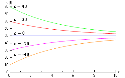
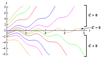
Back in the direction field section where we first derived the differential equation used in the last example we used the direction field to help us sketch some solutions. Let's see if we got them correct. To sketch some solutions all we need to do is to pick different values of c to get a solution. Several of these are shown in the graph below.

So, it looks like we did pretty good sketching the graphs back in the direction field section.
Now, recall from the Definitions section that the Initial Condition(s) will allow us to zero in on a particular solution. Solutions to first order differential equations (not just linear as we will see) will have a single unknown constant in them and so we will need exactly one initial condition to find the value of that constant and hence find the solution that we were after. The initial condition for first order differential equations will be of the form
y(t0)=y0$$y\left(t_0\right)=y_0$$Recall as well that a differential equation along with a sufficient number of initial conditions is called an Initial Value Problem (IVP).

Example 2 Solve the following IVP.dvdt=9.8−0.196vv(0)=48

Show Solution

v=50+ce−0.196t48=v(0)=50+c⇒c=−2v=50−2e−0.196t

Let’s do a couple of examples that are a little more involved.

Example 3 Solve the following IVP.cos(x)y′+sin(x)y=2cos3(x)sin(x)−1y(π4)=3√2,0≤x<π2

Show Solution

y′+sin(x)cos(x)y=2cos2(x)sin(x)−1cos(x)y′+tan(x)y=2cos2(x)sin(x)−sec(x)μ(t)=e∫tan(x)dx=eln|sec(x)|=elnsec(x)=sec(x)∫tan(x)dx=−ln|cos(x)|=ln|cos(x)|−1=ln|sec(x)|elnf(x)=f(x)sec(x)y′+sec(x)tan(x)y=2sec(x)cos2(x)sin(x)−sec2(x)(sec(x)y)′=2cos(x)sin(x)−sec2(x)∫(sec(x)y(x))′dx=∫2cos(x)sin(x)−sec2(x)dxsec(x)y(x)=∫sin(2x)−sec2(x)dxsec(x)y(x)=−12cos(2x)−tan(x)+cy(x)=−12cos(x)cos(2x)−cos(x)tan(x)+ccos(x)=−12cos(x)cos(2x)−sin(x)+ccos(x)3√2=y(π4)=−12cos(π4)cos(π2)−sin(π4)+ccos(π4)3√2=−√22+c√22c=7[Math Processing Error]y(x)=−12cos(x)cos(2x)−sin(x)+7cosx)(

Example 4 Find the solution to the following IVP.ty′+2y=t2−t+1y(1)=12

Show Solution

y′+2ty=t−1+1tμ(t)=e∫2tdt=e2ln|t|lnxr=rlnxμ(t)=e2ln|t|=eln|t|2=|t|2=t2(t2y)′=t3−t2+tt2y=∫t3−t2+tdt=14t4−13t3+12t2+cy(t)=14t2−13t+12+ct212=y(1)=14−13+12+c⇒c=112y(t)=14t2−13t+12+112t2

Example 5 Find the solution to the following IVP.ty′−2y=t5sin(2t)−t3+4t4y(π)=32π4

Show Solution

y′−2ty=t4sin(2t)−t2+4t3μ(t)=e∫−2tdt=e−2ln|t|μ(t)=e−2ln|t|=eln|t|−2=|t|−2=t−2(t−2y)′=t2sin(2t)−1+4tt−2y(t)=∫t2sin(2t)dt+∫−1+4tdtt−2y(t)=−12t2cos(2t)+12tsin(2t)+14cos(2t)−t+2t2+cy(t)=−12t4cos(2t)+12t3sin(2t)+14t2cos(2t)−t3+2t4+ct232π4=y(π)=−12π4+14π2−π3+2π4+cπ2=32π4−π3+14π2+cπ2π3−14π2=cπ2=π−14cy(t)=−12t4cos(2t)+12t3sin(2t)+14t2cos(2t)−t3+2t4+(π−14)t2

Let’s work one final example that looks more at interpreting a solution rather than finding a solution.

Example 6 Find the solution to the following IVP and determine all possible behaviors of the solution as t→∞. If this behavior depends on the value of y0 give this dependence.2y′−y=4sin(3t)y(0)=y0

Show Solution

y′−12y=2sin(3t)μ(t)=e∫−12dt=e−t2(e−t2y)′=2e−t2sin(3t)e−t2y=∫2e−t2sin(3t)dt+ce−t2y=−2437e−t2cos(3t)−437e−t2sin(3t)+cy(t)=−2437cos(3t)−437sin(3t)+cet2y0=y(0)=−2437+c⇒c=y0+2437y(t)=−2437cos(3t)−437sin(3t)+(y0+2437)et2

Range of c	Behavior of solution ast→∞
c < 0	y(t)→−∞
c = 0	y(t) remains finite
c > 0	y(t)→∞

Range of y0
y0<−2437	y(t)→−∞
y0=−2437	y(t) remains finite
y0>−2437	y(t)→∞

Investigating the long term behavior of solutions is sometimes more important than the solution itself. Suppose that the solution above gave the temperature in a bar of metal. In this case we would want the solution(s) that remains finite in the long term. With this investigation we would now have the value of the initial condition that will give us that solution and more importantly values of the initial condition that we would need to avoid so that we didn’t melt the bar.

from Fruitty Blog https://ift.tt/32CHNk7
via IFTTT